Producing
Products of Two Sets of Permutations
in Lexicographic Order
Jerry Bryan – 4 April 2023
I have been creating programs to investigate the mathematics of Rubik’s Cube since 1985. At various times since then, I have produced some rather long and convoluted descriptions of my methods. This document will be an attempt to clarify and shorten the description of one key part of my methods. In particular, this document will describe my method of producing the product of two sets of permutations in lexicographic order. As a consequence of the lexicographic ordering, it is possible to eliminate duplicate permutations and to count the number of unique permutations without storing any of the products in memory.
Let us suppose that we have two sets of permutation ![]() and
and ![]() . Forming all possible
products of
. Forming all possible
products of ![]() and
and ![]() will produce a list of
six products.
will produce a list of
six products.
![]()
We make two observations about this list of products. The
first observation is that we must treat the list as a sequence rather than as a
set because the list may contain duplicate permutations. For example, it is
possible that ![]() is the same permutation
as
is the same permutation
as ![]() . The second observation
is that simply forming the products by looping through the sets
. The second observation
is that simply forming the products by looping through the sets ![]() and
and ![]() will not produce the
products in lexicographic order. We will need to form the products in some
other way in order to produce them in lexicographic order.
will not produce the
products in lexicographic order. We will need to form the products in some
other way in order to produce them in lexicographic order.
There was a cube‑lovers mailing list which began in July 1980 and continued until January 2000. My method borrows from and builds upon two messages that were submitted to that mailing list.
The first message was from Alan Bawden. It described an algorithm which has become known as the Shamir Algorithm after its originator Adi Shamir. Bawden was reporting on the algorithm based on a lecture by Shamir. The algorithm provided a way to solve cube positions one at a time using very little computer memory during a timeframe when computers had very little memory. The message in the cube‑lovers archives may be found at the following URL:
Contained within the Shamir Algorithm was a method to produce products of permutations in lexicographic order. If you think of the method to solve a position as a theorem, then the method to produce products of permutations in lexicographic order might be considered a lemma. Lexicographic ordering of the product of two sets of permutations does not necessarily solve any problems on its own. However, lexicographic ordering of products can be useful as a part of various algorithms that actually do solve certain problems. The idea of producing products of two sets of permutations in lexicographic order is therefore a very powerful idea.
Bawden’s message about the Shamir Algorithm did not reflect
any computer code that implemented the algorithm. The algorithm was only
described as a concept. In addition, the message only described how to produce the
product ![]() in lexicographic order
for a sequence of permutations
in lexicographic order
for a sequence of permutations ![]() and for any particular
permutation
and for any particular
permutation ![]() . The process of combining
the sequences
. The process of combining
the sequences ![]() ,
, ![]() , … which are each in
lexicographic order into a combined sequence that is in lexicographic order was
left largely as an exercise for the reader.
, … which are each in
lexicographic order into a combined sequence that is in lexicographic order was
left largely as an exercise for the reader.
The article did suggest using a queue of items of the form ![]() with one item on the
queue for each
with one item on the
queue for each ![]() . The queue would be
ordered by the current
. The queue would be
ordered by the current ![]() from the
lexicographically ordered list
from the
lexicographically ordered list ![]() . The first element in the
queue would always be the first product currently in the queue in lexicographic
order. To get to the next element, the first element would be popped from the
queue and would be replaced in the queue by the next
. The first element in the
queue would always be the first product currently in the queue in lexicographic
order. To get to the next element, the first element would be popped from the
queue and would be replaced in the queue by the next ![]() for the
current
for the
current ![]() .
.
Using a queue to order the various ![]() items is not very
practical when both
items is not very
practical when both ![]() and
and ![]() might contain millions or
even billions of permutations. Too much time is spent popping one element off
the queue and inserting the element back into the queue in a different place. However,
the Shamir Algorithm was developed at a time when computer memories were so
small that it could be challenging to store even a few thousand permutations.
My method builds on Shamir’s original suggestion for producing products of
permutations in lexicographic order by providing an alternative to using a
queue. This alternative does scale up fairly well and is practical to use when
both
might contain millions or
even billions of permutations. Too much time is spent popping one element off
the queue and inserting the element back into the queue in a different place. However,
the Shamir Algorithm was developed at a time when computer memories were so
small that it could be challenging to store even a few thousand permutations.
My method builds on Shamir’s original suggestion for producing products of
permutations in lexicographic order by providing an alternative to using a
queue. This alternative does scale up fairly well and is practical to use when
both ![]() and
and ![]() contain very large
numbers of permutations.
contain very large
numbers of permutations.
The second message described an actual computer code which implemented the Shamir Algorithm. The message was posted by David Moews who was the author of the code. The message in the cube‑lovers archives may be found at the following URL:
The message from Moews included more details about the Shamir Algorithm
than had been posted before. It also included an improved method of combining
the various ![]() sequences into a single
list of permutations in lexicographic order. Namely, Moews merged all the
various
sequences into a single
list of permutations in lexicographic order. Namely, Moews merged all the
various ![]() sequences using Donald Knuth’s
Tournament of Losers Algorithm. My method builds further on the idea of
producing products of permutations in lexicographic order by eliminating
entirely the need to merge the various
sequences using Donald Knuth’s
Tournament of Losers Algorithm. My method builds further on the idea of
producing products of permutations in lexicographic order by eliminating
entirely the need to merge the various ![]() sequences. Instead, both
sequences. Instead, both ![]() and
and ![]() are partitioned in a
breadth first fashion that produces elements of
are partitioned in a
breadth first fashion that produces elements of ![]() in lexicographic order
without explicitly forming separate
in lexicographic order
without explicitly forming separate ![]() sequences that must then
be merged together.
sequences that must then
be merged together.
My model for lexicographic ordering is based on representing
permutations from words of an alphabet. For example, suppose our alphabet were ![]() a,b,c. Then each possible word
that is a permutation would contain exactly 3 letters, each possible word that
is a permutation would contain every letter in the alphabet, and no letter in
the alphabet would be repeated within a word that is a permutation. The list of
possible words that are permutations on the alphabet
a,b,c. Then each possible word
that is a permutation would contain exactly 3 letters, each possible word that
is a permutation would contain every letter in the alphabet, and no letter in
the alphabet would be repeated within a word that is a permutation. The list of
possible words that are permutations on the alphabet ![]() a,b,c are as follows.
a,b,c are as follows.
abc, acb, bac, bca, cab, cba
The lexicographic ordering is as if the words were ordered using the standard Latin alphabet from a to z.
My method to produce permutations in lexicographic tree does
not actually attempt to produce the product abc followed by the product acb followed
by the product bac, etc. Rather, the method walks a lexicographic
tree of the possible permutations that may be the product of any ![]() .
.
The easiest way to describe such a lexicographic tree is to show a picture of it. To that end, we will describe a notation for words from the alphabet when not all of the letters are known. We represent any unknown letter with a hyphen. For example, if the first two letters of a word are not known and the third letter is known to be b, we can write the word as ‑‑b. If the first and last letters of the word are not known and the second letter is known to be c, we can write the word as ‑c‑.
With that representation in mind, here is a lexicographic tree for all the words abc, acb, bac, bca, cab, cba when the words are listed in lexicographic order.
Figure 1.
Lexicographic Tree of ![]() a,b,c
a,b,c
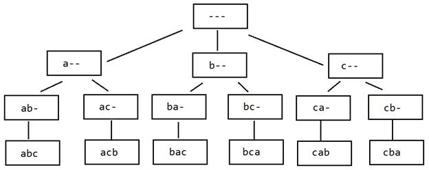
An immediate observation is that the last level of the tree is not necessary. For example, if we know that the first two letters of a word are ab then we know the third letter is c. Therefore, we define a lexicographic walk of the tree to be a depth first walk of the tree for level 0, level 1, and level 2 while omitting to walk at level 3. The child nodes to visit from each level are chosen in lexicographic order.
To make the lexicographic walk very explicit, the following
list of nodes shows the order in which the nodes are visited during a
lexicographic walk of this tree. Many of the nodes are visited more than one
time due to backtracking. We define ![]() as the sequence of nodes
visited during a lexicographic walk where
as the sequence of nodes
visited during a lexicographic walk where ![]() = ‑‑‑, a‑‑, ab‑, a‑‑, ac‑, a‑‑, ‑‑‑,
and so forth.
= ‑‑‑, a‑‑, ab‑, a‑‑, ac‑, a‑‑, ‑‑‑,
and so forth.
Figure 2
Lexicographic
Walk of ![]() a,b,c
a,b,c
tracking the path of λ = tree node
Action ![]()
1.
start ‑‑‑
2. down to a‑‑
3. down to ab‑
4. backtrack to a‑‑
5. down to ac‑
6. backtrack to a‑‑
7. backtrack to ‑‑‑
8. down to b‑‑
9. down to ba‑
10. backtrack to b‑‑
11. down to bc‑
12. backtrack to b‑‑
13. backtrack to ‑‑‑
14. down to c‑‑
15. down to ca‑
16. backtrack to c‑‑
17. down to cb‑
18. backtrack to c‑‑
19. backtrack to ‑‑‑
20. done
With this lexicographic walk in mind, we now can describe our method
as producing the products in ![]() via a lexicographic walk
rather than describing our method as producing products
via a lexicographic walk
rather than describing our method as producing products ![]() in lexicographic order.
The ultimate effect is the same either way. What is going on behind the curtain
is actually a depth first walk of the tree which has the effect of being a
lexicographic walk of the tree. We produce permutations that are elements of
in lexicographic order.
The ultimate effect is the same either way. What is going on behind the curtain
is actually a depth first walk of the tree which has the effect of being a
lexicographic walk of the tree. We produce permutations that are elements of ![]() via the equation
via the equation ![]() where
where ![]() takes on
each value in the lexicographic walk in turn.
takes on
each value in the lexicographic walk in turn.
For the most part it is ![]() that is taking the lead
and
that is taking the lead
and ![]() is just following. The
exception is when there is no
is just following. The
exception is when there is no ![]() and
and ![]() where the letters of the
product
where the letters of the
product ![]() match the current
match the current ![]() . In that case,
. In that case, ![]() follows
follows ![]() rather than leading
rather than leading ![]() . The effect is that
. The effect is that ![]() backtracks and as a
result of the backtracking it skips ahead. For example, if at step #2 of our
sample lexicographic walk there is no
backtracks and as a
result of the backtracking it skips ahead. For example, if at step #2 of our
sample lexicographic walk there is no ![]() and
and ![]() where the first letter of
the product
where the first letter of
the product ![]() is the letter a,
is the letter a, ![]() would skip ahead to step
#7 and the process would continue where the first letter of the product
would skip ahead to step
#7 and the process would continue where the first letter of the product ![]() would try to be the
letter b.
would try to be the
letter b.
For that reason, our equation ![]() might
better be written as the intersection
might
better be written as the intersection ![]() . When the intersection is
not null the method proceeds to the next node in the lexicographic walk
. When the intersection is
not null the method proceeds to the next node in the lexicographic walk ![]() . When the intersection is
null, the method backtracks which has the effect of skipping forward in the
lexicographic walk
. When the intersection is
null, the method backtracks which has the effect of skipping forward in the
lexicographic walk ![]() .
.
Thus far we have dealt with a permutation simply as a reordering
of the letters in words made from the 3 letters in the alphabet ![]() . We now need to treat a
permutation as a bijection on a set in order to be able to define the product
of two permutations. That is, we need to treat a permutation as a function or
mapping which is one‑to‑one and onto, and for which the domain and
range are the same set. We take the domain and range to be the alphabet
. We now need to treat a
permutation as a bijection on a set in order to be able to define the product
of two permutations. That is, we need to treat a permutation as a function or
mapping which is one‑to‑one and onto, and for which the domain and
range are the same set. We take the domain and range to be the alphabet ![]() .
.
With this definition of a permutation in mind, exactly what do
we mean by a permutation such as cab? We take cab to mean
that a as the
first letter of the alphabet ![]() is mapped to c, b as the
second letter of the alphabet
is mapped to c, b as the
second letter of the alphabet ![]() is mapped to a, and c as the
third letter of the alphabet
is mapped to a, and c as the
third letter of the alphabet ![]() is mapped to b. More
generally, suppose we have the permutation
is mapped to b. More
generally, suppose we have the permutation ![]() on the
alphabet
on the
alphabet ![]() where
where ![]() and
and ![]() are
unique letters from
are
unique letters from ![]() . We take
. We take ![]() to mean
that a as the
first letter of the alphabet
to mean
that a as the
first letter of the alphabet ![]() is mapped to
is mapped to ![]() , b as the
second letter of the alphabet
, b as the
second letter of the alphabet ![]() is mapped to
is mapped to ![]() , and c as the
third letter of the alphabet
, and c as the
third letter of the alphabet ![]() is mapped to
is mapped to ![]() .
.
For example, the permutation ![]() is defined as
is defined as ![]() and the permutation
and the permutation ![]() is defined as
is defined as ![]() . Therefore, the product
. Therefore, the product ![]() is the product
is the product ![]() which is
equal to
which is
equal to ![]() .
.
We are now prepared to have ![]() follow
follow ![]() . Suppose we are at step
#14 of the lexicographic walk where
. Suppose we are at step
#14 of the lexicographic walk where ![]() c‑‑.
We
need to find
c‑‑.
We
need to find ![]() and
and ![]() such that
such that ![]() c‑‑.
Remembering
that we must have
c‑‑.
Remembering
that we must have ![]() , there are 3 possible choices
we can make for Σ and Τ that are solutions.
, there are 3 possible choices
we can make for Σ and Τ that are solutions.
Figure 3
Choices for Σ and Τ
Σ
× Τ = ΣΤ
a‑‑ × c‑‑ = c‑‑
b‑‑ × ‑c‑ = c‑‑
c‑‑ × ‑‑c = c‑‑
We have arrived at the essential core of our method to produce
products of permutations in a way that follows a lexicographic walk. While ![]() is making a depth first
walk,
is making a depth first
walk, ![]() and
and ![]() are making their own
respective walks at the same time. The walks for
are making their own
respective walks at the same time. The walks for ![]() and
and ![]() must be breadth first
because we must process the product a‑‑ × c‑‑ at the
same time we process the product b‑‑ × ‑c‑
at
the same time we process the product c‑‑ × ‑‑c
= c‑‑. We cannot come back to process the separate products
at the same level of the walk later because that would put the values for
must be breadth first
because we must process the product a‑‑ × c‑‑ at the
same time we process the product b‑‑ × ‑c‑
at
the same time we process the product c‑‑ × ‑‑c
= c‑‑. We cannot come back to process the separate products
at the same level of the walk later because that would put the values for ![]() out of order.
out of order.
The computer code to implement our method is partitioning Σ and Τ. The code includes a performance enhancement that makes it easier to partition Τ. In addition to improving performance, the performance enhancement may perhaps make the method itself easier to understand. The performance enhancement takes advantage of the inverse identities such as the following. Using the inverses serves to place the letters of interest all in the same location within a word in Τ.
Figure 4
Inverse Identities
(c‑‑)‑1 = ‑‑a
(‑c‑)‑1 = ‑‑b
(‑‑c)‑1 = ‑‑c
Armed with these inverse identities, we can rewrite the values
for ![]() ,
, ![]() , and
, and ![]() at step #14 of the
lexicographic walk as follows.
at step #14 of the
lexicographic walk as follows.
Figure 5
Step #14 of the Lexicographic Walk
Σ
× Τ = ΣΤ
a‑‑ × (‑‑a)‑1 = c‑‑
b‑‑ × (‑‑b)‑1 = c‑‑
c‑‑ × (‑‑c)‑1 = c‑‑
The form of the lexicographic walk as portrayed in Figure #5
works because the permutations ‑‑a and ‑‑b and ‑‑c may be
taken to be τ‑1 values from the set ![]() , where
, where ![]() is the set of all
inverses of the set
is the set of all
inverses of the set ![]() . When we take the
inverses of the τ‑1 values, we are back to having τ values.
Therefore, to find permutations σ and τ whose product is c‑‑, the method
needs only to find pairs of permutations σ and τ where the first
letter of σ matches the third letter of τ‑1. That is
the performance enhancement of which we speak. It is much more efficient to
find matching letters in fixed locations in words than it is, for example, to
find the letter c no matter where it appears in a word. To facilitate
processing by inverses, the program stores all permutations as ordered pairs of
each permutation and its inverse. By storing the inverses, they do not need to
be calculated over and over again.
. When we take the
inverses of the τ‑1 values, we are back to having τ values.
Therefore, to find permutations σ and τ whose product is c‑‑, the method
needs only to find pairs of permutations σ and τ where the first
letter of σ matches the third letter of τ‑1. That is
the performance enhancement of which we speak. It is much more efficient to
find matching letters in fixed locations in words than it is, for example, to
find the letter c no matter where it appears in a word. To facilitate
processing by inverses, the program stores all permutations as ordered pairs of
each permutation and its inverse. By storing the inverses, they do not need to
be calculated over and over again.
I sometimes joke that the number of products of permutations that my programs produce is actually zero. That’s because my programs never calculate products. Instead, they match Σ and Τ in such a way that the desired products would be produced if they were actually calculated. Therefore, the matching serves the de facto function of forming the products without actually needing to form the products.
Proceeding from step #14 to step #15 of the lexicographic walk
for ![]() , the value of
, the value of ![]() is ca‑ and the
values for
is ca‑ and the
values for ![]() ,
, ![]() , and
, and ![]() would be as follows.
would be as follows.
Figure 6
Step #15 of the Lexicographic Walk
Σ
× Τ = ΣΤ
ab‑ × (b‑a)‑1 = ca‑
ac‑ × (c‑a)‑1 = ca‑
ba‑ × (a‑b)‑1 = ca‑
bc‑ × (c‑b)‑1 = ca‑
ca‑ × (a‑c)‑1 = ca‑
cb‑ × (b‑c)‑1 = ca‑.
We need to dig a little more deeply into how the lexicographic walk makes a transition from Step #14 in Figure 5 to Step #15 in Figure 6. We have already described how the walk would backtrack if there were no matches at all between the first letter of Σ and the third letter of Τ‑1. If there were a match, there could be matches on the letter a or the letter b or the letter c or some combination. Let’s suppose there was a match on the letter b and not on the letter a or the letter c. In that case, the status at Step #14 would be reduced to the following.
Figure 7
Step #14 of the Lexicographic Walk
without ΣΤ matches on the letters a or c
Σ
× Τ = ΣΤ
b‑‑ × (‑‑b)‑1 = c‑‑
Under these circumstances, the only matches brought forward would be the matches for the letter b. Therefore, the status at Step #15 of the lexicography walk would be the following.
Figure 8
Step #15 of the Lexicographic Walk
without ΣΤ matches brought forward on the letters a or c
as the first letter of Σ or the third letter of Τ‑1
Σ
× Τ = ΣΤ
ba‑ × (a‑b)‑1 = ca‑
bc‑ × (c‑b)‑1 = ca‑
There is a notational shortcut that greatly simplifies a description of the processing that takes place for Σ and Τ during the process of a lexicographic walk by λ. We represent the first letter of Σ and the matching letter in Τ‑1 by α and the second letter of Σ and the matching letter in Τ‑1 by β. It is understood that α is to be replaced in turn by each of a, b and c. It is understood that β is to be replaced in turnby each of the letters not assigned to α.
Σ and Τ are still processed breadth first, but the breadth first aspect of the processing is hidden in the notation. Additional Greek letters would be used in the same fashion for an alphabet of more than 3 letters.
Figure 9
Step #14 of the Lexicographic Walk
with and without shortcut notation
Σ
× Τ = ΣΤ
without
shortcut notation
a‑‑ × (‑‑a)‑1 = c‑‑
b‑‑ × (‑‑b)‑1 = c‑‑
c‑‑ × (‑‑c)‑1 = c‑‑
with shortcut notation
α‑‑ × (‑‑α)‑1 = c‑‑
Figure 10
Step #15 of the Lexicographic Walk
with and without shortcut notation
Σ
× Τ = ΣΤ
without
shortcut notation
ab‑ × (b‑a)‑1 = ca‑
ac‑ × (c‑a)‑1 = ca‑
ba‑ × (a‑b)‑1 = ca‑
bc‑ × (c‑b)‑1 = ca‑
ca‑ × (a‑c)‑1 = ca‑
cb‑ × (b‑c)‑1 = ca‑
with
shortcut notation
αβ‑ × (β‑α)‑1 = ca‑
The shortcut notation greatly facilitates an understanding of the computer code that implements this method to produce products of permutations in lexicographic order. The corners of Rubik’s Cube are represented by words from an alphabet of 24 letters from a to x. The edges of Rubik’s Cube are represented by words from second alphabet of 24 letters from a to x. Therefore, the actual lexicographic walks conducted by the computer code are vastly larger than the simple example in this document using an alphabet of only 3 letters. The maximum number of permutations in Σ and Τ that the computer code can handle on a typical desktop class computer is about 108. Therefore, the maximum number of products of permutations the computer code can handle on a typical desktop class computer is about 1016. That requires a much longer lexicographic walk than the simple one displayed in Figure 2.
That being said, we will conclude this document by repeating the short lexicographic walk from Figure 2. Except this time, we will use the shortcut notation to describe the behavior of Σ and Τ along with the behavior of λ.
Figure 11
Lexicographic Walk of ω= a,b,c
tracking the path of Σ, Τ, and λ
Action λ ∩ Σ × Τ
1. start ‑‑‑
∩ -‑‑ × ‑‑‑-1
2. down to a‑‑
∩ α‑‑ × α‑‑-1
3. down to ab‑
∩ αβ‑ × αβ‑-1
4. backtrack to a‑‑ ∩
α‑‑ × α‑‑-1
5. down to ac‑
∩ αβ‑ × α‑β-1
6. backtrack to a‑‑ ∩
α‑‑ × α‑‑-1
7. backtrack to ‑‑‑
∩ ‑‑‑ × ‑‑‑-1
8. down to b‑‑
∩ α‑‑ × ‑α‑-1
9. down to ba‑
∩ αβ‑ × βα‑-1
10. backtrack to b‑‑ ∩
α‑‑ × ‑α‑-1
11. down to bc
∩ αβ‑ × ‑αβ-1
12. backtrack to b‑‑ ∩
α‑‑ × ‑α‑-1
13. backtrack to ‑‑‑
∩ ‑‑‑ × ‑‑‑-1
14. down to c‑‑
∩ α‑‑ × -‑α-1
15. down to ca‑
∩ αβ‑ × β‑α-1
16. backtrack to c‑‑ ∩
α‑‑ × -‑α-1
17. down to cb‑
∩ αβ‑ × -βα-1
18. backtrack to c‑‑ ∩
α‑‑ × -‑α-1
19. backtrack to -‑‑ ∩
‑‑‑ × ‑‑‑-1
20.
done
Added 7 April 2023. Despite this document including the word “lexicographic” in its title, the walk portrayed in Figure 11 does not actually need to be lexicographic in order to achieve its desired effect of creating a walk that visits each possible product of permutations at most one time. For example, we can think of the walk as of containing three sub-walks: steps 2 through 7, steps 8 through 13, and steps 14 through 19. We could perform sub-walk 8 through 13 first, sub-walk 14 through 19 second, and sub-walk 2 through 7 last. If so, the new walk would still allow us to visit produce all the products of permutations in Σ and Τ in such a way that we could identify and eliminate products that were duplicate without needing to store any of the products in memory. Similarly, steps 9 through 10 and steps 11 through 12 are sub-walks that could be formed in either order.
Such a non-lexicographic walk can be useful when distributing a large Rubik’s Cube problem across multiple processor cores on a single machine or across multiple machines. For example, a sub-walk such as steps 2 through 7 could be processed on one computer, a sub-walk such as steps 8 through 13 could be processed on a second computer, and a sub-walk such as steps 14 through 19 could be processed on a third computer. The sub-walks on the separate computers would be much longer than the very short sub-walks in this example. Nevertheless, the concept is the same with very long sub-walks as with short sub-walks.